Tutorial#
Sometimes, in high contrast direct imaging observations, background objects can masquerade as planet candidates. These confounding sources reveal their true nature over time. Since direct imaging targets are typically bright, foreground stars with large proper motions, they move much, much faster than the typical background star, and their proper motion difference, added to the parallactic motion of the Earth causes them to follow a helical path.
A classical test in high contrast imaging is the “common proper motion” test, comparing the relative path of a source to a helical background track to test whether the source is consistent with being bound to the host star or fixed to the background frame.
A pathological case can arise when a background star has a non-zero parallax or fast proper motions of its own. In this case, it is necessary, but not sufficient, to demonstrate that the source doesn’t follow the infinite-distance, stationary background track. It takes longer and typically higher precision data to detect helical motion from moving background sources that are at a finite distance.
This tutorial will show the user how to calculate the simple case, an infinite distance stationary background track for a quick comparison, and then to fit a model for the pathological finite distance, moving background track to data.
The curious case of HD 131339 A “b”#
Start by downloading the astrometry data on the companion candidate around HD 131339 A to the local working folder. This data was compiled from Wagner et al. (2016), Nielsen et al. (2017), and with additional observations from Wagner et al. (2022, data priv. comm.). Our analysis of the dataset follows Nielsen et al., but backtracks improves on the previous
analysis in a few small ways (mostly leveraging updated Gaia DR3 information).
Formatting input relative astrometry#
This .csv file is formatted following orbitize! (documentation here), specifically their “epoch, object, quant1, quant1_err, quant2, quant2_err, quant12_corr, quant_type” formatting. Mesurements are assumed to be in milliarcseconds [mas] or degrees (for positon angles). You can specify relative astrometry as “radec” or “seppa” using the quant_type column, and if these measurements do not have a correlation, quant12_corr
can be set to nan. Even if your .csv input contains only measurements for a single candidate, it is important to have the 2nd column be the “object” column, where the value is 1 for the entire range of measurements. If you have a file with more than one candidate’s astrometry recorded, set the keyword argument “obj_num” to the integer of the object you’re currently examining (see an example
here). The only distinction from the orbitize! format is that object = 0 can refer to a candidate you have labeled as “0”, and does not refer to the host star (whose parameters are set implicitly by backtracks, except for host star RV which can be specified manually).
[1]:
!wget https://github.com/wbalmer/backtracks/raw/refs/heads/main/tests/scorpions1b_orbitizelike.csv
--2026-03-30 17:16:06--  https://github.com/wbalmer/backtracks/raw/refs/heads/main/tests/scorpions1b_orbitizelike.csv
Resolving github.com (github.com)... 140.82.112.4
Connecting to github.com (github.com)|140.82.112.4|:443... connected.
HTTP request sent, awaiting response... 302 Found
Location: https://raw.githubusercontent.com/wbalmer/backtracks/refs/heads/main/tests/scorpions1b_orbitizelike.csv [following]
--2026-03-30 17:16:06--  https://raw.githubusercontent.com/wbalmer/backtracks/refs/heads/main/tests/scorpions1b_orbitizelike.csv
Resolving raw.githubusercontent.com (raw.githubusercontent.com)... 185.199.108.133, 185.199.109.133, 185.199.111.133, ...
Connecting to raw.githubusercontent.com (raw.githubusercontent.com)|185.199.108.133|:443... connected.
HTTP request sent, awaiting response... 200 OK
Length: 831 [text/plain]
Saving to: ‘scorpions1b_orbitizelike.csv.10’

scorpions1b_orbitiz 100%[===================>]     831  --.-KB/s    in 0s

2026-03-30 17:16:06 (79.3 MB/s) - ‘scorpions1b_orbitizelike.csv.10’ saved [831/831]
Initialization#
Then, import the System class from the backtracks package.
[2]:
from backtracks import System
Now, we can set up the System class. We’ll provide it with:
the Simbad resolvable name of our host star of interest
target_name=[your star's name]a .csv file containing the relative positions of our candidate source around our host star (
candidate_file=[your .csv file here, see the example .csv for an example).a range in degrees around which we’ll construct a local sample of proper motions and parallaxes from Gaia (
nearby_window=0.5, the default is 0.5 degrees, which is fine for most cases)a path to a directory to save our figures and intermediate data products (
fileprefix=[your/path/here/])
[3]:
track = System(target_name="HD 131399 A",
               candidate_file="scorpions1b_orbitizelike.csv",
               nearby_window=0.5,
               fileprefix='./')
[BACKTRACKS INFO]: Examining object = 1 in input file.
[BACKTRACKS INFO]: Resolved the target star 'HD 131399 A' in Simbad!
[BACKTRACKS INFO]: Resolved target's Gaia ID from Simbad, Gaia DR3 6204835284262018688
INFO: Query finished. [astroquery.utils.tap.core]
[BACKTRACKS INFO]: gathered Gaia DR3 data for HD 131399 A
   * Gaia source ID = 6204835284262018688
   * Reference epoch = 2016.0
   * RA = 223.6053 deg
   * Dec = -34.1429 deg
   * PM RA = -30.70 mas/yr
   * PM Dec = -30.77 mas/yr
   * Parallax = 9.75 mas
   * RV = 15.61 km/s
INFO: Query finished. [astroquery.utils.tap.core]
[BACKTRACKS INFO]: gathered 6445 Gaia objects from the 0.5 sq. deg. nearby HD 131399 A
[BACKTRACKS INFO]: Finished nearby background gaia statistics
[BACKTRACKS INFO]: Queried distance prior parameters, L=2524.23, alpha=1.05, beta=0.62
[BACKTRACKS INFO]: Estimating candidate position if stationary in RA,Dec @ 2016.0 from observation #0
[BACKTRACKS INFO]: Opened ephemeris file
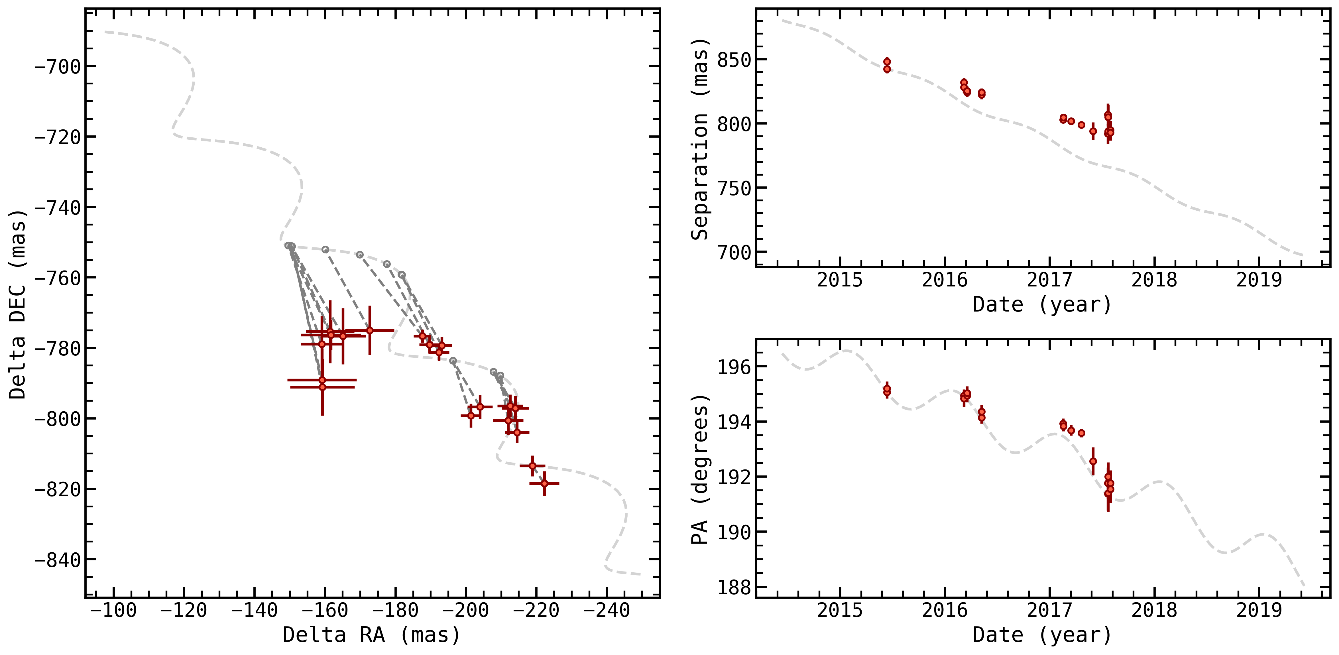
The backtracks.System class queries Simbad, then Gaia and retrieves both the Gaia parameters for the host star and the distribution of parameters for all the stars nearby (this is useful for quantifying whether your candidate’s motion is an outlier in terms of velocity or distance). It then sets up the stationary, infinite distance background object case, and compares the data to this track. Let’s take a look at that visually:
Stationary, infinite distance background track#
[4]:
fig_stationary = track.generate_stationary_plot(days_backward=1.*365.,
                                                days_forward=4.*365,
                                                step_size=10.,
                                                filepost='.png')
[BACKTRACKS INFO]: Generating Stationary plot
[BACKTRACKS INFO]: Stationary track reduced chi squared is 29.30
[BACKTRACKS INFO]: Stationary plot saved to ./
Generate arrays of RA, Dec for a given set of parameters and times#
While we like to think our built in plots are pretty great, you can use backtracks to generate arrays of RA and Dec for a given set of parameters on a given array of times, so that you can create your own visualizations or analyses. You just need to initialize a System and pass the system, an array of julian days (in terrestrial time), and an array of parameters to backtracks.utils.radecdists.
[5]:
import numpy as np
import matplotlib.pyplot as plt
from astropy.time import Time
from backtracks.utils import radecdists, utc2tt
# create an array of times
projected_epochs = np.arange(Time('2015-06-12').jd, Time('2017-01-12').jd, 1)
projected_epochs_tt = utc2tt(projected_epochs)

# we need an array of parameters, which are
# ra, dec, pmra, pmdec, par, ra_host, dec_host, pmra_host, pmdec_host, par_host, rv_host
# in many cases, we're just interested in the stationary case, so we can pull the array of those parameters directly from our System
parameters = track.stationary_params

# now, we just call the System.radecdists function
ras, decs = radecdists(track, projected_epochs_tt, parameters) # these array have units mas

# and we'll plot the results to prove this works
plt.figure(figsize=(4,4))
plt.plot(ras, decs, c='k', zorder=-1)

plt.xlim(-160, -230)
plt.ylim(-825, -765)

# and we can throw up some data
plt.errorbar(track.ras[0:6], track.decs[0:6], yerr=track.decserr[0:6], xerr=track.raserr[0:6],
             color="tomato",ecolor='darkred', linestyle="none",
             marker='o', ms=5., mew=1.5, mec='darkred')

# and label the axes
plt.xlabel('$\Delta$RA (mas)')
plt.ylabel('$\Delta$Dec (mas)')

plt.show()
<>:30: SyntaxWarning: invalid escape sequence '\D'
<>:31: SyntaxWarning: invalid escape sequence '\D'
<>:30: SyntaxWarning: invalid escape sequence '\D'
<>:31: SyntaxWarning: invalid escape sequence '\D'
/var/folders/z3/sbzzx8w10cx6yd_63fg3nngm0000gn/T/ipykernel_24194/1374084939.py:30: SyntaxWarning: invalid escape sequence '\D'
  plt.xlabel('$\Delta$RA (mas)')
/var/folders/z3/sbzzx8w10cx6yd_63fg3nngm0000gn/T/ipykernel_24194/1374084939.py:31: SyntaxWarning: invalid escape sequence '\D'
  plt.ylabel('$\Delta$Dec (mas)')
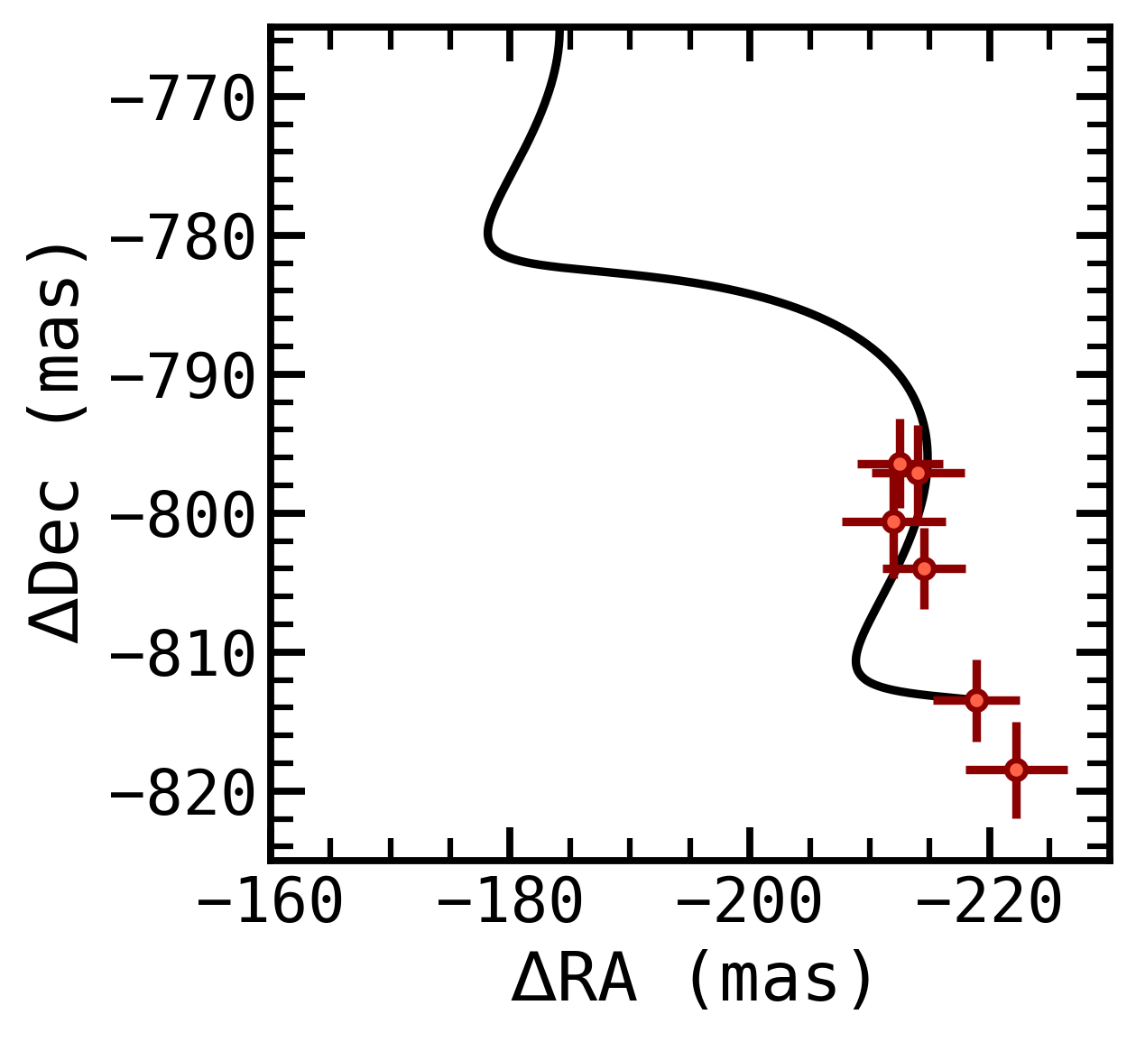
It looks like the stationary, infinite distance case is a pretty poor fit to this data. Does that mean these are observations of a planet?! Unfortunately, no. The fit is poor, but the data and this helical motion share some visual similarities that might prompt us to consider continuing to use backtracks to investigate.
Fitting for moving, finite distance background tracks#
We can set up and run a fit that will use the nested sampling package dynesty to explore varying the proper motion and parallax of a background star, and compare this apparent helical motion to our data.
fit takes a number of parameters, not all of which you might care about at the start. You can set any combination of these parameters to:
sample more coarsely (lower nlive), or more finely (increase nlive)
speed up convergence but sacrifice precision (increase dlogz, e.g. to 1 or 10).
use more cpu cores (set npool higher)
sample the posterior fully (set dynamic=True) but note that this can take a while!
run on a cluster with mpi_pool = True
resume from a previous run
or, depending on your case, to speed up convergence on a different dataset 7) use a different sampling method (e.g. ‘rwalk’ or ‘rslice’)
Let’s run a coarse, initial fit that will terminate rather early to get a handle on the results of backtracks. For a more accurate assessment, we’d recommend you use more live points nlive=1000, and we’d recommend exploring dynamic sampling to flesh out your posterior distribution with dynamic=True. Note that if your data is not well described by helical background track motion, these fits will struggle to converge, so we recommend you always start by comparing your data to the
stationary case, and run a coarse, easily terminated inital run before spending computation time on a full fit.
[6]:
results = track.fit(nlive=400,
                    dlogz=0.1,
                    npool=4,
                    dynamic=False,
                    mpi_pool=False,
                    resume=False,
                    sample_method='unif'
                   )
[BACKTRACKS INFO]: Beginning sampling
iter: 10549 | +400 | bound: 121 | nc: 1 | ncall: 65435 | eff(%): 16.836 | loglstar: -inf < -99.740 < inf | logz: -123.753 +/- 0.236 | dlogz: 0.000 > 0.100
Save and load results#
We’ll save our results to disk, so that we can access them without re-running the sampler:
[7]:
track.save_results(fileprefix='./')
[BACKTRACKS INFO]: Saving results to ./HD_131399_A_cc1_dynestyrun_results.pkl
And we can load those results (initializing the track object with the System class in the same way as above):
[8]:
track.load_results(fileprefix='./')
[BACKTRACKS INFO]: Loading results from ./HD_131399_A_cc1_dynestyrun_results.pkl
Plotting your fit#
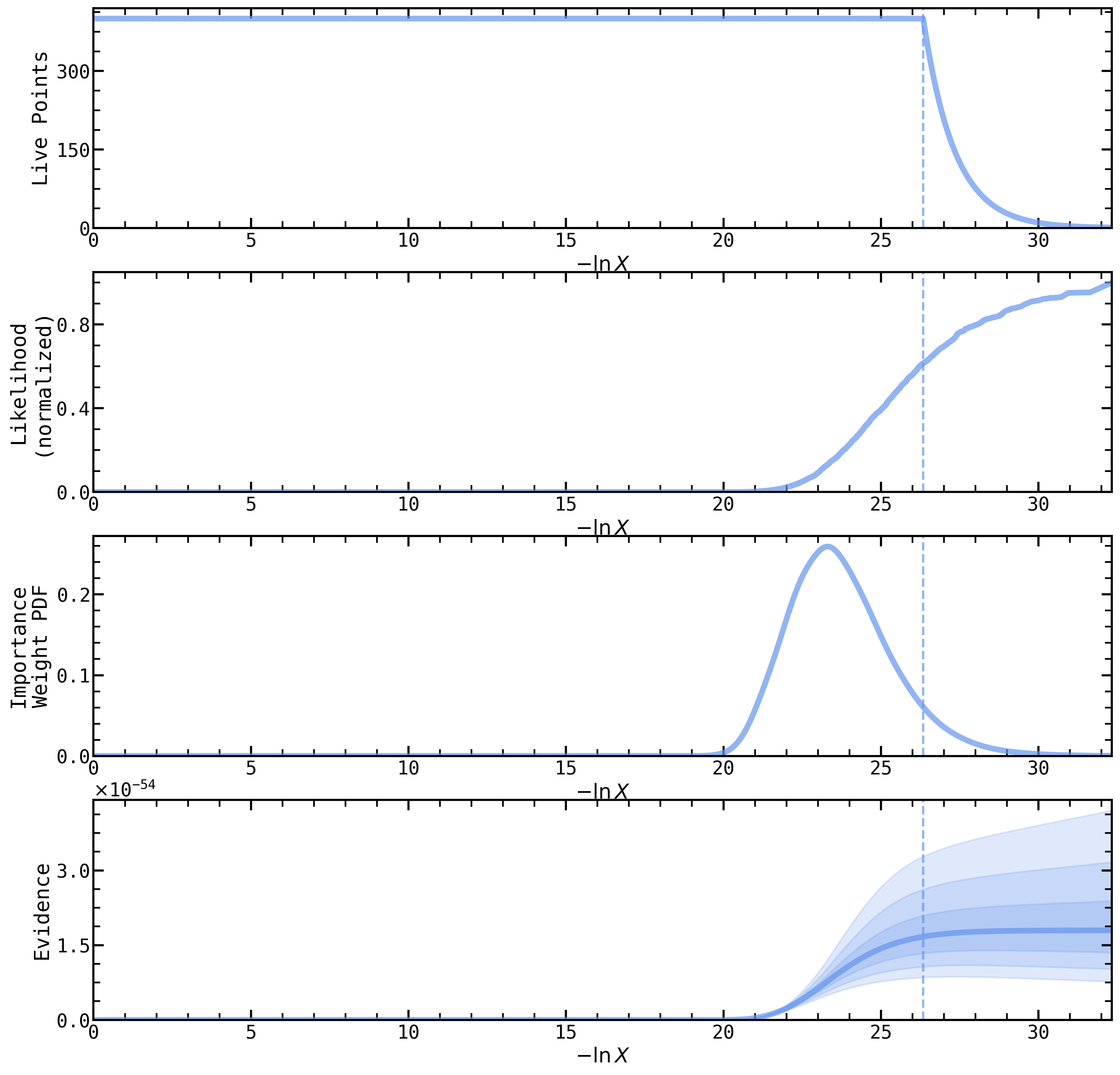
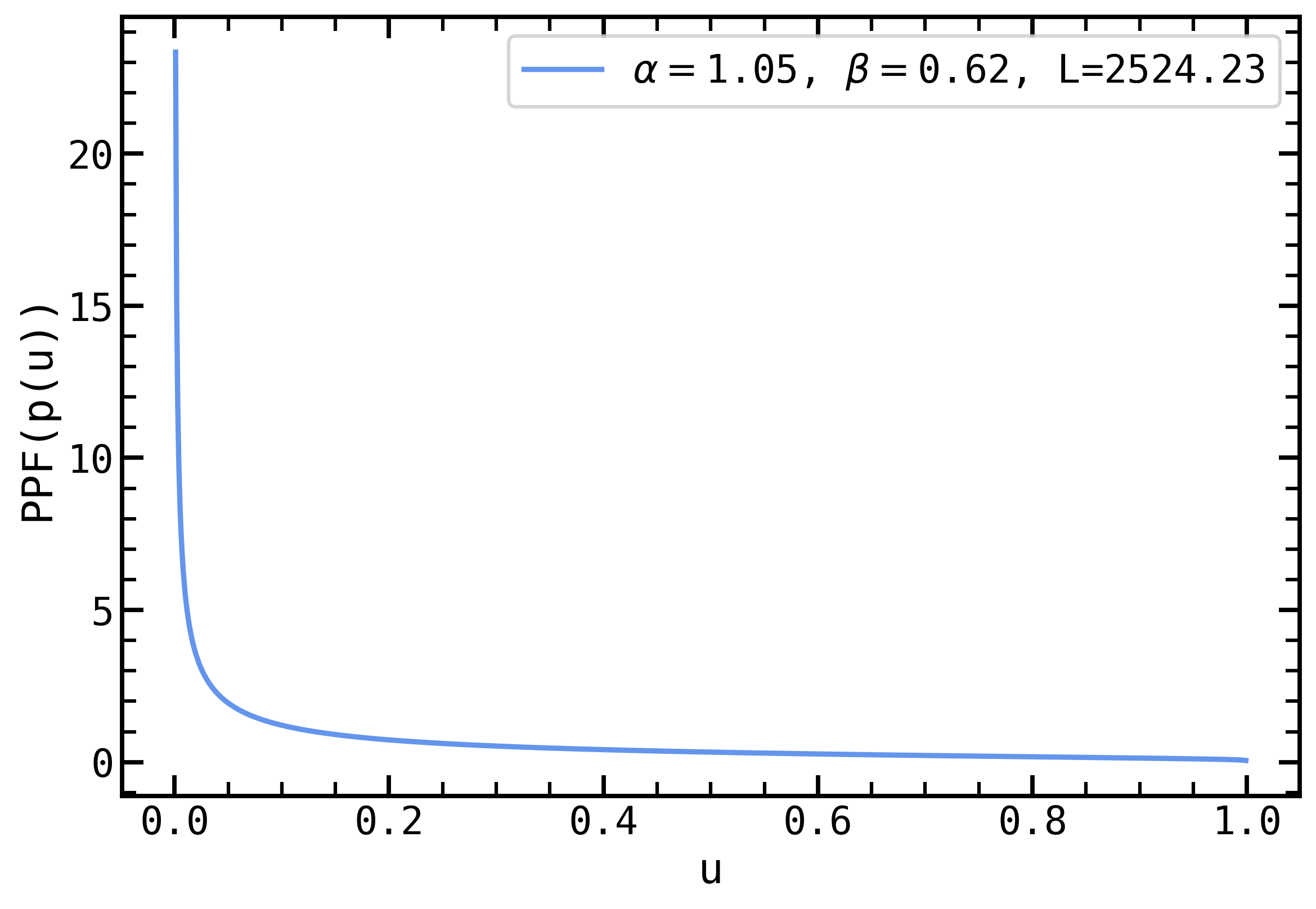
You can then plot the results of your fit using the functions in backtracks.plotting. We have two convenience functions within the System class to generate these plots with a single line of code (the first of which we used above to generate the stationary track plot). We’ll generate a plot of the visual helix, a plot of the posterior distribution of parameters, a plot of diagnostics for the dynesty sampler run, a plot showing the prior on parallax we’ve assumed, and a plot of our
median sample compared to the distribution of nearby Gaia measurements.
[ ]:
fig_track, fig_post, fig_diag, fig_prior, fig_hood = \
    track.generate_plots(days_backward=1.*365.,
                         days_forward=4.*365,
                         step_size=10.,
                         plot_radec=False,
                         plot_stationary=True,
                         fileprefix='./',
                         filepost='.png')
[BACKTRACKS INFO]: Generating Plots
[BACKTRACKS INFO]: Stationary track reduced chi squared is 29.30
[BACKTRACKS INFO]: Median track reduced chi squared is 0.68
/Users/wbalmer/codebank/backtracks/backtracks/plotting.py:81: RuntimeWarning: divide by zero encountered in divide
  ppf = 1000./transform_gengamm(u, backtracks.L, backtracks.alpha, backtracks.beta)
[BACKTRACKS INFO]: Plots saved to ./
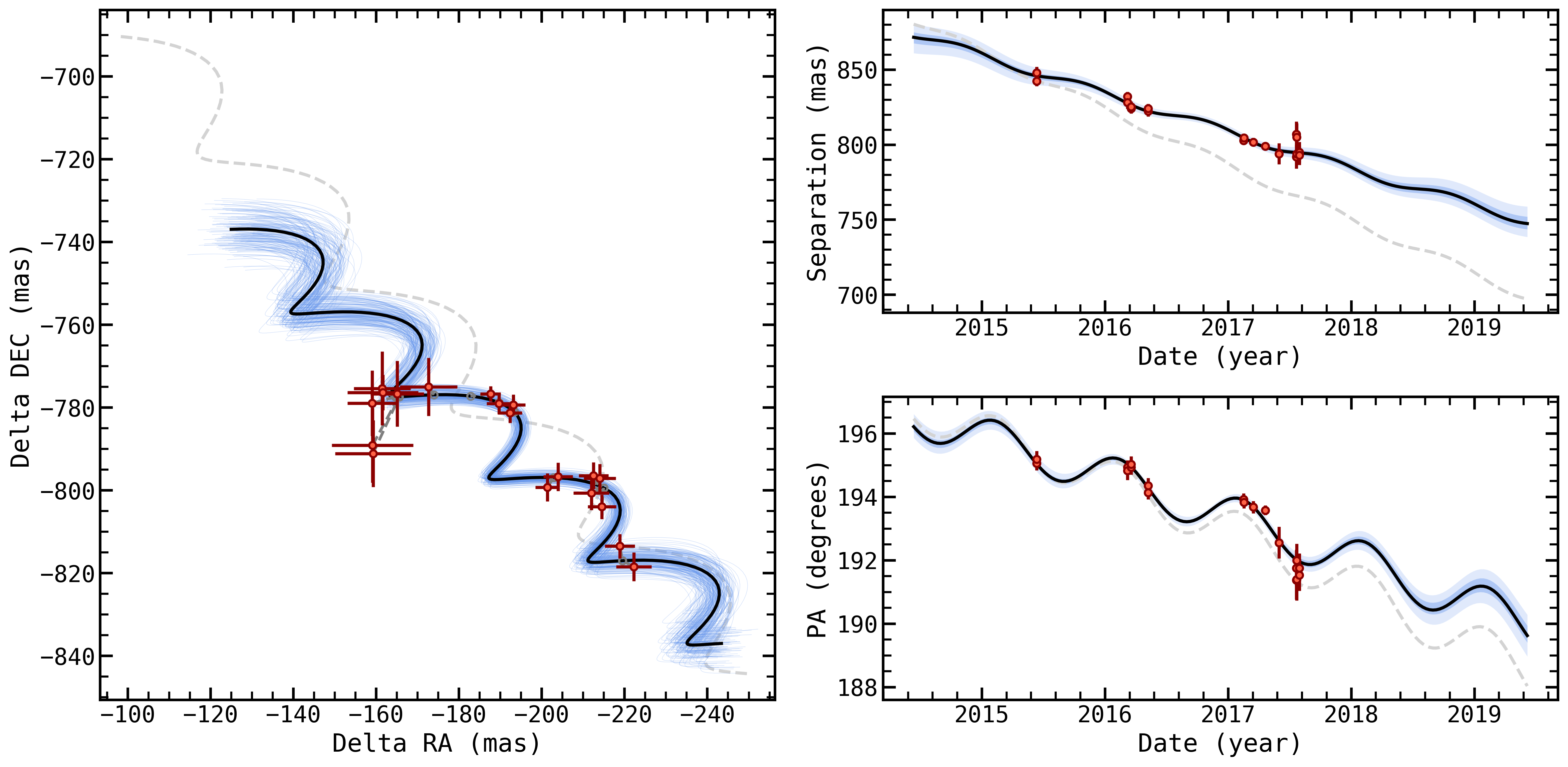
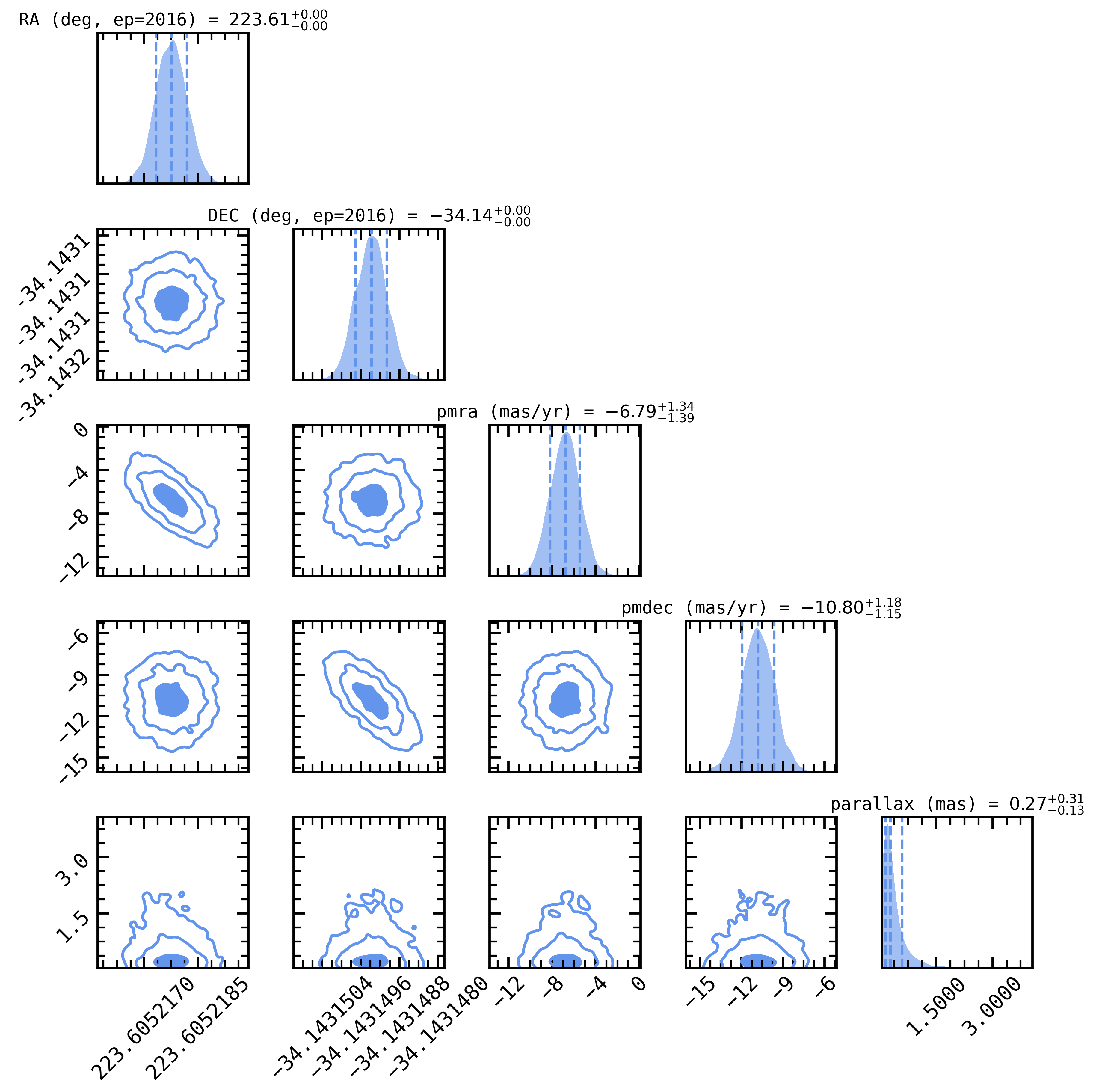
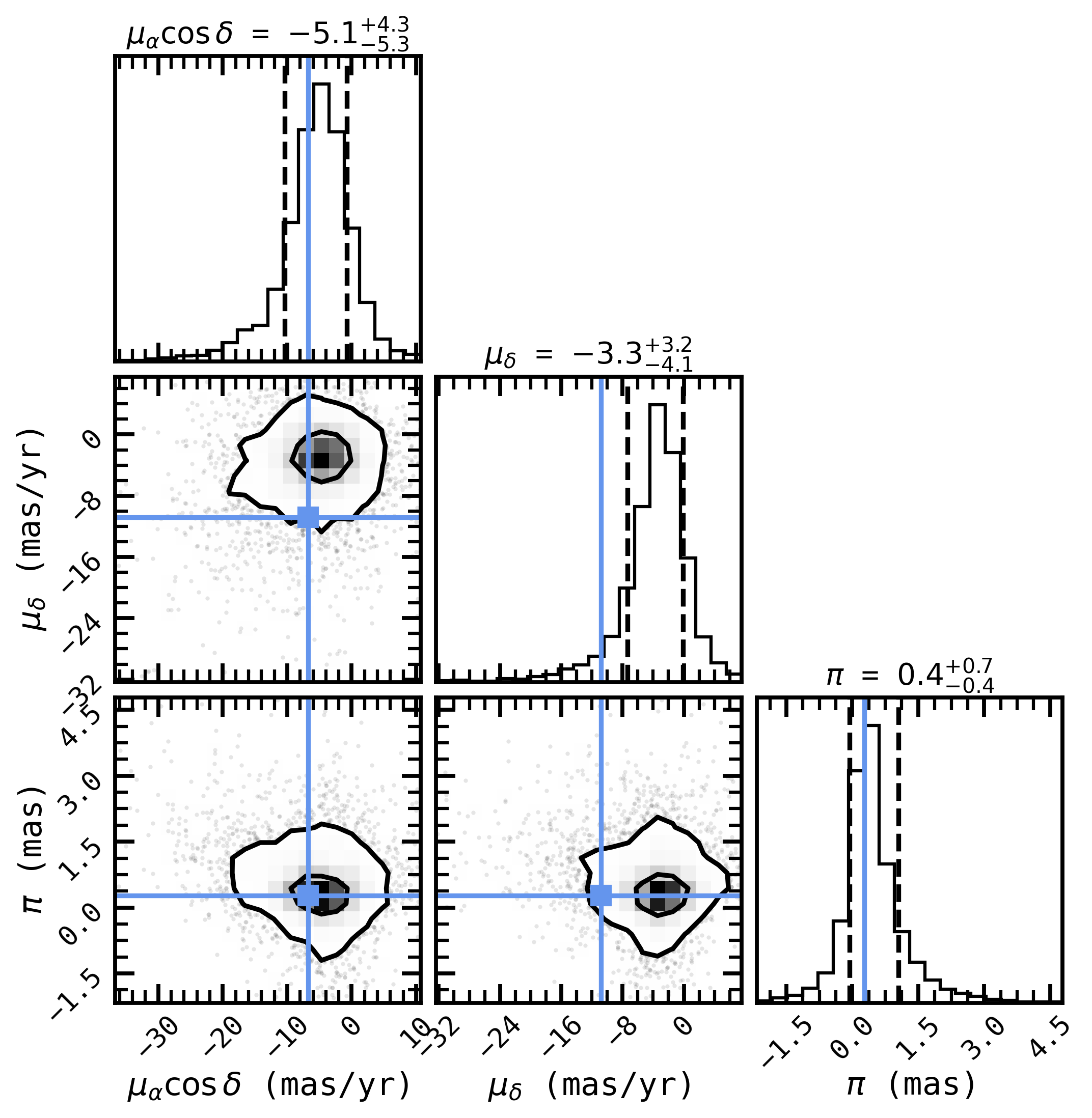
Unfortunately for HD131339 Ab, it looks like the data is well fit by a distant, quickly moving background star (as it turns out, the candidate’s spectral energy distribution is also well fit by stellar spectral types). We’ve just reproduced a key result of Nielsen et al. (2017)’s argument (see their figure 19). If we were to publish this result, we’d probably want to increase our number of live points (or use dynamic nested sampling) to fully sample the posterior and be sure of our final numbers.
What next?#
Depending on the result of backtracks.System.fit, you could compare the goodness of fit between the median of this posterior distribution of background star cases to that of a bound, planetary orbit to decide whether your candidate is a planet or not. You can access the samples, or the median sample, from the System object via System.results.samples, and report the goodness of fit with System.median_chi2_red.
In the case where there is little curvature in your data, and backtracks.System.fit reproduces effectively linear motion with the same parallax as the host, that’s pretty good evidence that you have a bound body (a planet!) on your hands. We’d recommend using orbitize! or another orbit fitting package to assess this case, and compare to your backtracks results. If the motion is poorly fit by both a bound orbit and a moving, finite distance background track, then something even
weirder might be going on.
Feel free to reach out to the developers (William, Gilles, and Tomas) if you run into any trouble using the code, or if you’d like advice on any particular use cases.